Hierarchical clustering procedures can be agglomerative and divisive. In the agglomerative method classification starts from maximal number of groups which corresponds number of cases, that is every case considered as one group. Then the cases are sequentially combined into similar groups. Clustering procedure step-by-step links more and more objects together and amalgamates larger and larger clusters with increasingly dissimilar elements until only one cluster is left.
The divisive method forms clusters just in opposite way: all observations are initially assumed to belong to a single cluster, and then the most dissimilar observations are extracted one-by-one to form separate clusters.
The agglomerative method is more common. During formation of clusters, dissimilarities or distances between them are calculated. The results are expressed not only in numerical statistics but also in hierarchical tree diagram called dendrogram which shows the linkage point:

Linkage distance is shown in horizontal or vertical axe depending on type of dendrogram. In the above the dendrogram is horizontal and horizontal lines correspond similarity distance between clusters, which are linked at each stage. Each node in the dendrogram shows the point where a new cluster is formed, and looking at distance axe we can determine the criterion distance at which the respective elements were grouped together into a new single cluster. The clusters are linked at increasing levels of dissimilarities (distances) and so number of produced groups is different depending on distance point:

For example, at figure above all cases can be grouped into fours clusters by using relative distance equal to 10, or to two clusters if distance equal to 15 is used:

Appropriate number of clusters can be chosen by researchers themselves taking into account application of results to the experimental data.
Hierarchical clustering is based on calculation of matrix of all possible distances between cases. In large database, which contains tens of thousands of cases, it may take too much time and because of this, this method is not always applicable.
The purpose of cluster analysis is the objective classification of cases. However, there are different methods to measure distance between cases and to choose between which points these distances are measured, which finally may significantly influence results of classification and bring some subjectivism. Because of this, during describing results of cluster analysis it is always necessary to mention distance measure and clustering algorithm.
Distance can be expressed in variety of ways. For comparison, distance between two cities can be geographical and expressed in kilometres, or can be as ‘level of progress’ calculated from population, number of internet-users, cars, etc. In the first case, two capital cities from different continents are located farther from each other than from some town in the same country; however, accordingly to the second measurement, these capitals are closer to each other, than to the neighbouring village. In cluster analysis also there are distance which just express geometric distance and there are distances which measure other criteria, for example correlation coefficient.
Like with the Two-step clustering and k-means clustering, we will discuss performing hierarchical cluster analysis in SPSS using example with sensitivity of different bacteria to 42 antibiotics (see Example 7).
Performing hierarchical cluster analysis in SPSS
1) Click the Analyze menu, point to Classify, and select Hierarchical Cluster… :
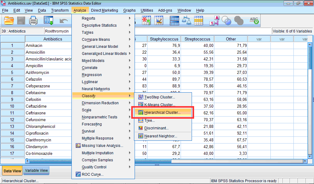
The Hierarchical Cluster Analysis dialog box opens:
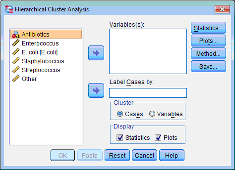
2) Select the variables on which classification of objects will be based (“Enterococcus”, “E.coli”, “Staphylococcus”, “Streptococcus”, “Other”); click the upper transfer arrow button  . The selected variables are moved to the Variable(s): list box.
3) During examination of dendrogram it is more convenient when case labels are expressed. For this purpose select the variable “Antibiotics”, which contains names of antibiotics, then click the lower transfer arrow button  . The selected variables are moved to the Label Cases by: list box.
4) Click the Statistics… button; the Hierarchical Cluster Analysis: Statistics dialog box opens:
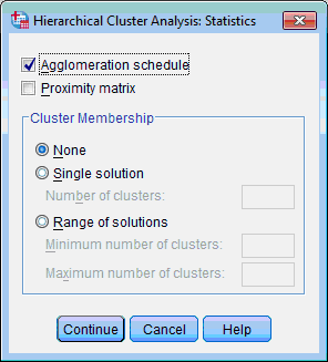
5) By default only the Agglomeration Schedule check box is selected. Select also the Proximity Matrix check box. Click the Continue button. This returns you to the Hierarchical Cluster Analysis dialog box.
6) To express dendrogram among clustering results click the Plots… button; Hierarchical Cluster Analysis: Plots dialog box opens:
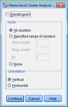
7) Select the Dendrogram check box. Other options leave selected by default. Click the Continue button. This returns you to the Hierarchical Cluster Analysis dialog box.
8) Click the Method… button; the Hierarchical Cluster Analysis: Methods dialog box opens:
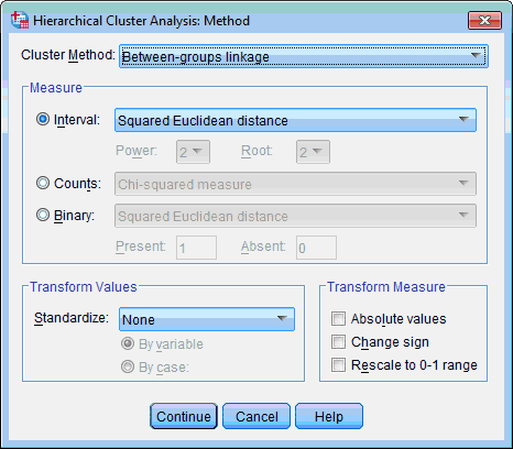
In this dialog box we can choose clustering method (algorithm), distance measure and if necessary perform transformation of our data. Also we may use options proposed by default (between-groups linkage algorithm and squared Euclidian distance). Click the Continue button. This returns you to the Hierarchical Cluster Analysis dialog box.
9) In the Cluster section of Hierarchical Cluster Analysis dialog box we may choose, whether clustering of cases or variables should be performed. Our example supposes clustering of cases which is chosen by default.
10) In the Display section of Hierarchical Cluster Analysis dialog box we may select displaying of statistics or/and plots among results. By default both options are selected.
11) Click the OK button. An Output Viewer window opens and displays the results.
Results of hierarchical clustering analysis are presented in three tables, Case Processing Summary (contains only number of valid, missing and total cases), Proximity Matrix and Agglomeration Schedule, and in two charts – Vertical (or Horizontal) Icicle and Dendrogram. Both icicle plot and dendrogram can be either vertical or horizontal, but it is sometimes more convenient to interpret horizontal ones when there are many cases.
The Proximity Matrix table contains matrix of distances between all cases:
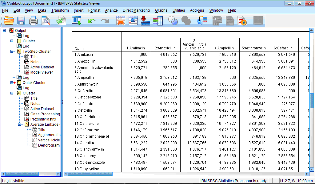
Number of rows and columns is equal to number of cases and if many cases present it becomes rather difficult to interpret it. From the fragment of this matrix presented in Fig. 8.35 we can see that, for example, distance (difference) between “Amikacin” and “Amoxicillin” is bigger than difference between “Amikacin” and “Clindamycin”: the corresponding values of squared Euclidian distances are 4042.552 and 590.142.
The Agglomeration schedule table describes process of grouping of the cases:
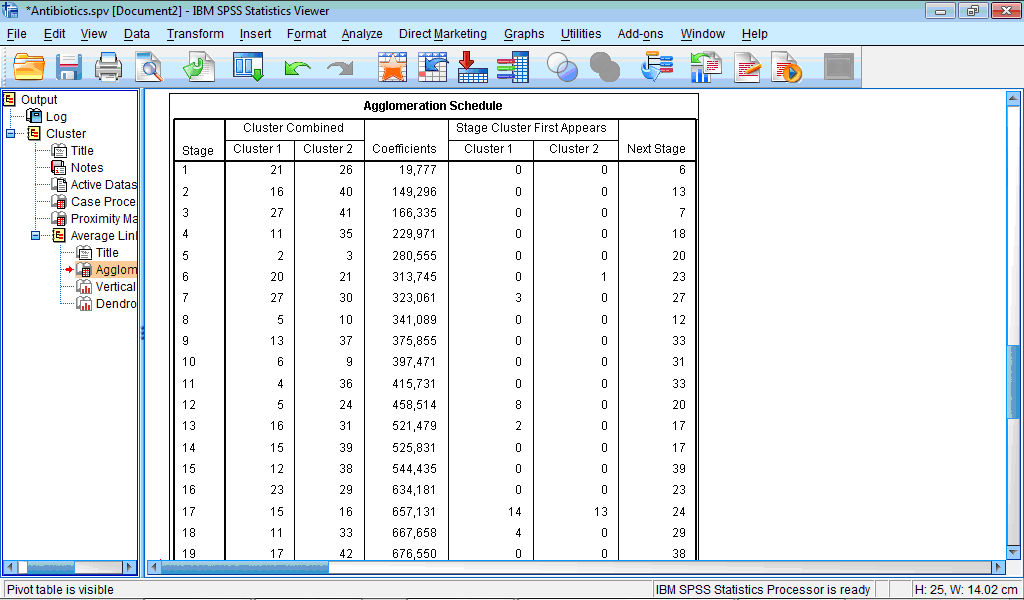
The column Stage shows number of clustering stage; the column Cluster Combined shows which clusters are combined at each stage; column Coefficients contains values of distance measure for every combined cases or clusters, in our example, these are values of squared Euclidian distance; column Stage Cluster First Appears shows ‘history of clustering’, that is, at which stage cluster 1 and cluster 2 previously appeared in this table; and, finally, last column Next Stage shows at which stage this new cluster will be further proceeded.
For example, in our table first line (Stage 1) shows that first of all cases 21 and 26 are combined with squared Euclidian distance 19.777. Values “0” in both columns for Stage Cluster First Appears show that previously these cases were not grouped with any other cases. Column Next Stage shows that this cluster will be further grouped at stage 6. Let us now look now at Stage 6: here case 20 and cluster containing case 21 are grouped together with squared Euclidian distance of 313.745. We also can see that case 20 was not previously grouped anywhere (value “0” in the column Stage Cluster First Appears), while case 21 was already grouped with another cases as stage 1 (value “1” in this column). Further this new cluster, containing now cases 20, 21 and 26, will be grouped with the next case (or cluster) at the stage 23.
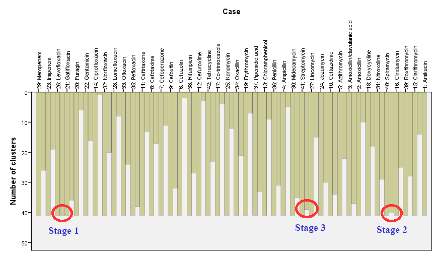
The icicle plot got such name because in case of vertical icicle plot produced columns look like icicles hanging from the eaves. The icicle plot gives information about combining cases into clusters at each step of clustering; it graphically displays the information on agglomeration schedule. Near each case there are two columns – longer and shorter, for interpretation is used the shorter one. It is read ‘from bottom to up’: at beginning we have 42 clusters, when individual cases correspond to separate clusters; this stage is not shown. Then first two cases are grouped and after this we will have 41 clusters, it corresponds the longest columns – between cases “Levofloxacin” (case 26) and “Gatifloxacin” (case 21) ( ‘Stage 1’). At the next stage cases “Spiramycin” (case 40) and “Clindamycin” (case 16) are grouped (‘Stage 2’), after this we will have 40 clusters, which we can see at the vertical axe on the left scale. At the third stage cases “Streptomycin” (41) and “Lincomycin” (27) are grouped, and so on until the last free case (“Ciprofloxacin” – cases 14) will be grouped with cluster containing case 32 “Norfloxacin” (and all other cases previously attached to this cluster):
Dendrogram gives similar information but in another view. We can can see stages of combining cases into clusters, but its branching-type nature allows tracing backward or forwarding any individual case or clustering at any level. Dendrogram contains the scale corresponding distance between cases and clusters which gives information about similarity between them. The dendrogram is read from left to right: we can see consecutive grouping of individual cases into clusters:
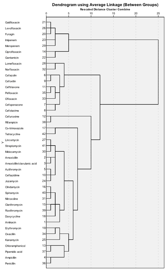
From the dendrogram we can see that first seven antibiotics in upper part of it (gatifloxacin, levofloxacin, furagin, imipenem, meropenem, ciprofloxacin and gentamicin) are combined into separate cluster, in contrast to all other antibiotics. Looking into the table with original data, it becomes clear that this cluster contains the most active antibiotics.
In summary, comparing three clustering methods, we can see that resulting classifications are similar to some extent when the purpose is to select the most ‘extreme’ cases. Number of groups and their characteristics are easily detected in two-step and k-means clustering; however, inner structure of dataset can be revealed in the best way by hierarchical cluster analysis.

